Shaking Table System Testing and Verification

5.1 Test Platform

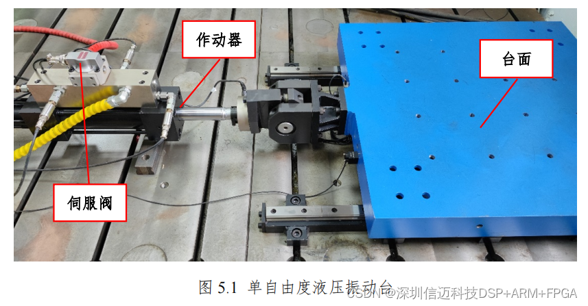
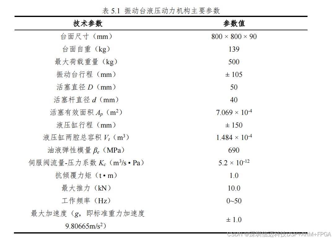
Figure 5.1 shows the single-degree-of-freedom electro-hydraulic servo shaking table used in this paper, with its main parameters listed in Table 5.1.

5.2 Data Preprocessing

The controller architecture designed in this paper is relatively general-purpose. The motion waveform can be a sine wave, a random wave, or an earthquake wave. In experiments where the reference waveform is an earthquake wave, data preprocessing is required. Two scenarios here require preprocessing: one is when earthquake wave data only contains acceleration waveforms, without displacement and velocity waveforms. In this case, velocity and displacement need to be synthesized from acceleration, and baseline correction may be necessary [50]; the second scenario is when displacement, velocity, and acceleration reference waveform data are all available, but the frequency is low and the number of points is sparse, for example, one point every 5ms. In this case, interpolation based on existing data is required. Most earthquake waves downloaded from the earthquake database website (https://esm-db.eu/) have displacement, velocity, and acceleration data, but the points are not dense enough, falling into the second scenario. Therefore, before the experiment, the earthquake wave data is preprocessed with interpolation to convert it to one reference point every 1ms.

5.2.1 Cubic Spline Interpolation

Cubic spline interpolation is a special type of piecewise cubic interpolation. It only has two more boundary conditions at the endpoints of the interpolation interval compared to Lagrange interpolation, but its first and second derivatives are continuous at the internal nodes, making it smoother than piecewise Hermite cubic interpolation [51].

5.2.2 Interpolation Effect

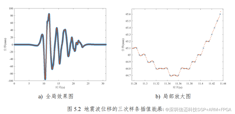
Taking an earthquake wave data from Romania (earthquake ID RO-1977-0001) as an example, cubic spline interpolation is performed, and the interpolation result of its displacement waveform is shown in Figure 5.2.

5.3.2 Sine Wave Test

Figure 5.3 shows the real-time display of the sine wave test results on the host computer, where the green line represents the reference waveform and the red line represents the actual collected waveform. The sine wave frequency is 2Hz, and the amplitude is 50mm. The host computer software supports exporting and saving waveform data. Figure 5.4 shows the processing results of the waveform data exported by the host computer.

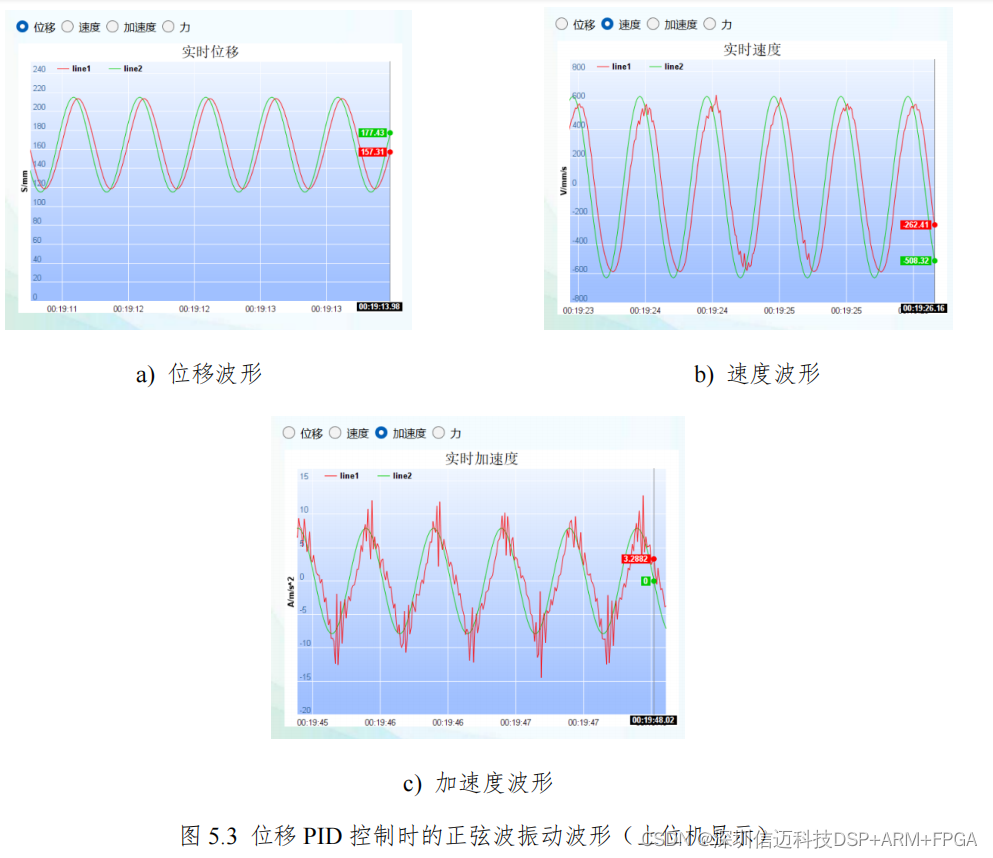
After calculation, the harmonic distortion of the displacement waveform is 0.02%, the harmonic distortion of the velocity waveform is 0.21%, and the harmonic distortion of the acceleration waveform is 2.02%. The correlation coefficient of the displacement waveform is 99.86%, the correlation coefficient of the velocity waveform is 98.85%, and the correlation coefficient of the acceleration waveform is 94.87%. Considering that in vibration tests, general time offset does not substantially affect the testing of materials or structures, the time lag is subtracted when calculating the correlation coefficient.